The dataset for this exercise can be found here
>getwd()
>setwd("C:/Users/joyis/Downloads")
>bcancer<-read.csv("Breast_cancer_data.csv")
>summary(bcancer)
mean_radius      mean_texture   mean_perimeter     mean_area
 Min.   : 6.981   Min.   : 9.71   Min.   : 43.79   Min.   : 143.5
 1st Qu.:11.700   1st Qu.:16.17   1st Qu.: 75.17   1st Qu.: 420.3
 Median :13.370   Median :18.84   Median : 86.24   Median : 551.1
 Mean   :14.127   Mean   :19.29   Mean   : 91.97   Mean   : 654.9
 3rd Qu.:15.780   3rd Qu.:21.80   3rd Qu.:104.10   3rd Qu.: 782.7
 Max.   :28.110   Max.   :39.28   Max.   :188.50   Max.   :2501.0
 mean_smoothness   diagnosis
 Min.   :0.05263   0:212
 1st Qu.:0.08637   1:357
 Median :0.09587
 Mean   :0.09636
 3rd Qu.:0.10530
 Max.   :0.16340
>head(bcancer)
mean_radius mean_texture mean_perimeter mean_area mean_smoothness diagnosis
1 17.99 10.38 122.80 1001.0 0.11840 0
2 20.57 17.77 132.90 1326.0 0.08474 0
3 19.69 21.25 130.00 1203.0 0.10960 0
4 11.42 20.38 77.58 386.1 0.14250 0
5 20.29 14.34 135.10 1297.0 0.10030 0
6 12.45 15.70 82.57 477.1 0.12780 0>tail(bcancer)
mean_radius mean_texture mean_perimeter mean_area mean_smoothness diagnosis
564 20.92 25.09 143.00 1347.0 0.10990 0
565 21.56 22.39 142.00 1479.0 0.11100 0
566 20.13 28.25 131.20 1261.0 0.09780 0
567 16.60 28.08 108.30 858.1 0.08455 0
568 20.60 29.33 140.10 1265.0 0.11780 0
569 7.76 24.54 47.92 181.0 0.05263 1>str(bcancer)
'data.frame': 569 obs. of 6 variables:
$ mean_radius : num 18 20.6 19.7 11.4 20.3 ...
$ mean_texture : num 10.4 17.8 21.2 20.4 14.3 ...
$ mean_perimeter : num 122.8 132.9 130 77.6 135.1 ...
$ mean_area : num 1001 1326 1203 386 1297 ...
$ mean_smoothness: num 0.1184 0.0847 0.1096 0.1425 0.1003 ...
$ diagnosis : Factor w/ 2 levels "0","1": 1 1 1 1 1 1 1 1 1 1 ...
>install.packages("caret")

>install.packages("class")
>install.packages("gmodels")
>install.packages("plotly")
>install.packages('e1071')
>bcancer$diagnosis<-as.factor(bcancer$diagnosis)
>fig<-plot_ly(data=bcancer, x = ~mean_area, y=~mean_radius, color = ~diagnosis)
>fig
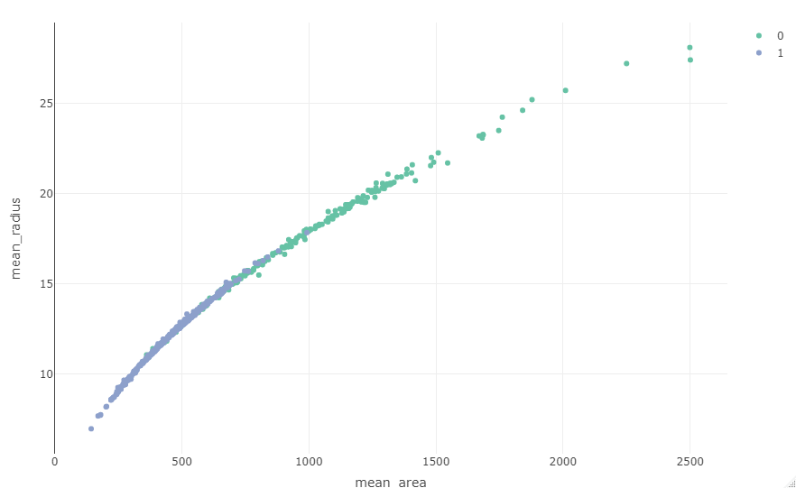
>fig2<-plot_ly(data=bcancer, x = ~mean_perimeter, y=~mean_radius, color = ~diagnosis)
>fig2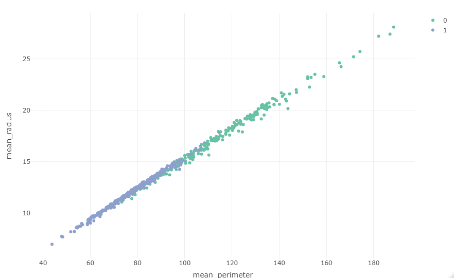
fig3<-plot_ly(data=bcancer, x = ~mean_perimeter, y=~mean_texture, color = ~diagnosis)
fig3
>set.seed(3465)
>bc <- sample(2, nrow(bcancer), replace=TRUE, prob=c(0.7, 0.3))

# use the sample that is stored in the variable bc to define the training and test sets
>bcancerTrain <- bcancer[bc==1, 1:5]
>bcancerTest <- bcancer[bc==2, 1:5]
>bcancerTrainLabels <- bcancer[bc==1, 6]
>bcancerTestLabels <- bcancer[bc==2, 6]
>bcancer_pred <- knn(train = bcancerTrain, test = bcancerTest, cl = bcancerTrainLabels, k=3)
CrossTable(x=bcancerTestLabels, y= bcancer_pred, prop.chisq = F)Total Observations in Table: 179
| bcancer_pred
bcancerTestLabels | 0 | 1 | Row Total |
------------------|-----------|-----------|-----------|
0 | 52 | 13 | 65 |
| 0.800 | 0.200 | 0.363 |
| 0.852 | 0.110 | |
| 0.291 | 0.073 | |
------------------|-----------|-----------|-----------|
1 | 9 | 105 | 114 |
| 0.079 | 0.921 | 0.637 |
| 0.148 | 0.890 | |
| 0.050 | 0.587 | |
------------------|-----------|-----------|-----------|
Column Total | 61 | 118 | 179 |
| 0.341 | 0.659 | |
------------------|-----------|-----------|-----------|
The table shows that 13 out of 65 negative breast cancer diagnoses were incorrectly grouped as positive and 9 positive results out of 105 were incorrectly grouped as negative. I repeated the analysis using a 0.9 and 0.1 ratio.
bcancer$diagnosis
bc2 <- sample(2, nrow(bcancer), replace=TRUE, prob=c(0.9, 0.1)) # 90% and 10%
# use the sample that is stored in the variable bc2 to define the training and test sets
bcancerTrain2 <- bcancer[bc2==1, 1:5]
bcancerTest2 <- bcancer[bc2==2, 1:5]
bcancerTrainLabels2 <- bcancer[bc2==1, 6]
bcancerTestLabels2 <- bcancer[bc2==2, 6]
bcancer_pred2 <- knn(train = bcancerTrain2, test = bcancerTest2, cl = bcancerTrainLabels2, k=3)


CrossTable(x=bcancerTestLabels2, y= bcancer_pred2, prop.chisq = F)
Total Observations in Table:  57


                   | bcancer_pred2
bcancerTestLabels2 |         0 |         1 | Row Total |
-------------------|-----------|-----------|-----------|
                 0 |        18 |         4 |        22 |
                   |     0.818 |     0.182 |     0.386 |
                   |     0.900 |     0.108 |           |
                   |     0.316 |     0.070 |           |
-------------------|-----------|-----------|-----------|
                 1 |         2 |        33 |        35 |
                   |     0.057 |     0.943 |     0.614 |
                   |     0.100 |     0.892 |           |
                   |     0.035 |     0.579 |           |
-------------------|-----------|-----------|-----------|
      Column Total |        20 |        37 |        57 |
                   |     0.351 |     0.649 |           |
-------------------|-----------|-----------|-----------|
The table shows that 2 out of 35 positive breast cancer diagnoses were incorrectly grouped as negative and 4 negative results were incorrectly grouped as positive.
Caret Analysis
#Caret Analysis
>bcancer$diagnosis<-as.factor(bcancer$diagnosis)
>set.seed(3000)
>btrain_test<-createDataPartition(y= bcancer$diagnosis, p= 0.7, list = FALSE)
>btraining_data<-bcancer[btrain_test,]  #70% of data used for training
>btesting_data<-bcancer[-btrain_test,]  #30% of data used for testing
#The train control method was implemented
>btrain_control<-trainControl(method = "repeatedcv", number=10, repeats = 3)
>str(btraining_data)
'data.frame':	399 obs. of  6 variables:
 $ mean_radius    : num  20.6 19.7 11.4 12.4 13.7 ...
 $ mean_texture   : num  17.8 21.2 20.4 15.7 20.8 ...
 $ mean_perimeter : num  132.9 130 77.6 82.6 90.2 ...
 $ mean_area      : num  1326 1203 386 477 578 ...
 $ mean_smoothness: num  0.0847 0.1096 0.1425 0.1278 0.1189 ...
 $ diagnosis      : Factor w/ 2 levels "0","1": 1 1 1 1 1 1 1 1 1 1 ...
>svm_bcancer <- train(diagnosis~., data = btraining_data, method="svmLinear",
trControl=btrain_control,
preProcess=c("center", "scale"), tuneLength= 10)
>svm_bcancerSupport Vector Machines with Linear Kernel
399 samples
5 predictor
2 classes: '0', '1'
Pre-processing: centered (5), scaled (5)
Resampling: Cross-Validated (10 fold, repeated 3 times)
Summary of sample sizes: 359, 359, 359, 359, 359, 359, ...
Resampling results:
Accuracy Kappa
0.9173077 0.8224182
Tuning parameter 'C' was held constant at a value of 1#After running the "svm_analysis", my result showed a C value of 1. This means that it is a linearly separable value.
#I created and ran my test_prediction code and checked for accuracy of predictions using the confusion matrix.
>test_predictionbcancer<-predict(svm_bcancer, newdata= btesting_data)
>confusionMatrix(table(test_predictionbcancer, btesting_data$diagnosis))Accuracy : 0.9353
95% CI : (0.8872, 0.9673)
No Information Rate : 0.6294
P-Value [Acc > NIR] : <2e-16
Kappa : 0.8599
Mcnemar's Test P-Value : 0.5465
Sensitivity : 0.8889
Specificity : 0.9626
Pos Pred Value : 0.9333
Neg Pred Value : 0.9364
Prevalence : 0.3706
Detection Rate : 0.3294
Detection Prevalence : 0.3529
Balanced Accuracy : 0.9258
'Positive' Class : 0 #To improve the accuracy of my model, I customized the cost value of my linear classification. I inputted values for C using the code:
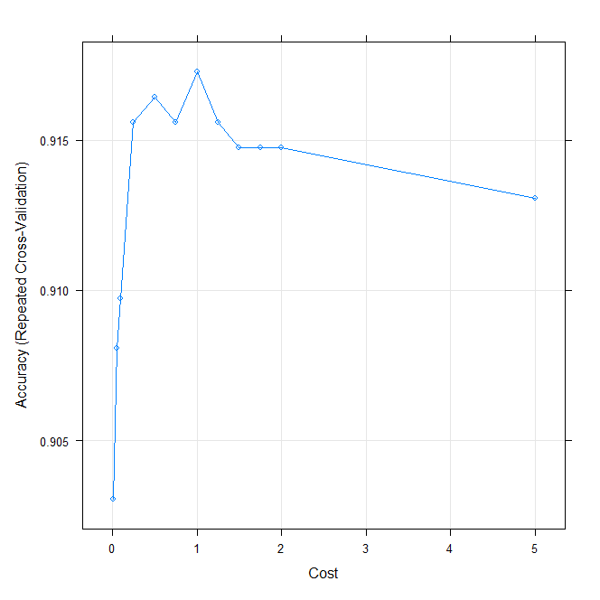
>grid<-expand.grid(C=c(0,0.01,0.05,0.1,0.25,0.5,0.75, 1, 1.25, 1.5,1.75,2,5))
>svm_analysis_grid<-train(diagnosis~., data=btraining_data, method="svmLinear",
trControl=btrain_control, preProcess = c("center", "scale"),
tuneGrid= grid, tuneLength = 10)Pre-processing: centered (5), scaled (5)
Resampling: Cross-Validated (10 fold, repeated 3 times)
Summary of sample sizes: 359, 359, 359, 359, 360, 359, ...
Resampling results across tuning parameters:
C Accuracy Kappa
0.00 NaN NaN
0.01 0.9030556 0.7812334
0.05 0.9080556 0.7979656
0.10 0.9097222 0.8033340
0.25 0.9155769 0.8181449
0.50 0.9164316 0.8201596
0.75 0.9155769 0.8185886
1.00 0.9172650 0.8219160
1.25 0.9155983 0.8185380
1.50 0.9147436 0.8165419
1.75 0.9147436 0.8165419
2.00 0.9147436 0.8165419
5.00 0.9130769 0.8129364
Accuracy was used to select the optimal model using the largest value.
The final value used for the model was C = 1.>plot(svm_analysis_grid)
#Testing Phase
#After training the model, I tested it with the following code:
>bcancermodel_test_grid<-predict(svm_analysis_grid,newdata=btesting_data)
>table(bcancermodel_test_grid)
bcancermodel_test_grid
0 1
60 110