The dataset can be obtained here

The Heart dataset was analyzed using the simple linear regression method.

The heart dataset comprises of the following variables:

Age: The Age of the patients in years.

Sex: The sex of the patients (1 = male, 0 = female)

Chest_Pain_Type: The chest pain type experienced by the patients (Value 1: typical angina, Value 2: atypical angina, Value 3: non-anginal pain, Value 4: asymptomatic)

Resting_BP: The person’s resting blood pressure (mm Hg on admission to the hospital)

Serum_Cho: The person’s cholesterol measurement in mg/dl

High_Fbs: The person’s fasting blood sugar (> 120 mg/dl, 1 = true; 0 = false)

Resting_ECG: Resting electrocardiographic measurement (0 = normal, 1 = having ST-T wave abnormality, 2 = showing probable or definite left ventricular hypertrophy by Estes’ criteria)

Heart_Rate_Max: The patient’s maximum heart rate achieved.

Ex_Ang: Exercise induced angina? (1 = yes; 0 = no)

Old_Peak: ST depression induced by exercise relative to rest.

Slope: Slope of the peak exercise ST segment (Value 1: upsloping, Value 2: flat, Value 3: downsloping)

FCBV: The number of major vessels colored by flourosopy (0-3)

Thal: A blood disorder called thalassemia (3 = normal; 6 = fixed defect; 7 = reversable defect)

Diagnosis: Heart disease (0 = no, 1 = yes)

Data Analysis

library(‘psych’)
>Heart_data<- read.csv(“heart_data.csv”)
headTail(Heart_data)

## Age Sex Chest_Pain_Type Resting_BP Serum_Cho High_FBS Resting_ECG
## 1 70 1 4 130 322 0 2
## 2 67 0 3 115 564 0 2
## 3 57 1 2 124 261 0 0
## 4 64 1 4 128 263 0 0
## ... ... ... ... ... ... ... ...
## 267 44 1 2 120 263 0 0
## 268 56 0 2 140 294 0 2
2
## 269 57 1 4 140 192 0 0
## 270 67 1 4 160 286 0 2
## Heart_Rate_Max Ex_Ang Old_Peak Slope FCBV Thal Diagnosis
## 1 109 0 2.4 2 3 3 2
## 2 160 0 1.6 2 0 7 1
## 3 141 0 0.3 1 0 7 2
## 4 105 1 0.2 2 1 7 1
## ... ... ... ... ... ... ... ...
## 267 173 0 0 1 0 7 1
## 268 153 0 1.3 2 0 3 1
## 269 148 0 0.4 2 0 6 1
## 270 108 1 1.5 2 3 3 2

library('PerformanceAnalytics')
library('corrplot')
library('dplyr')
new_data<-cor(select(Heart_data, 1:4, 10:14))
round(new_data,3)
corrplot.mixed(cor(new_data), order='hclust', tl.col='black')
>new_data<-cor(select(Heart_data, 1:4, 10:14))
>round(new_data,3)
##      Age   Sex  Chest_Pain_Type Resting_BP Old_Peak Slope FCBV
## Age 1.000 -0.094 0.097 0.273 0.194 0.160 0.356
## Sex -0.094 1.000 0.035 -0.063 0.097 0.051 0.087
## Chest_Pain_Type 0.097 0.035 1.000 -0.043 0.167 0.137 0.226
## Resting_BP 0.273 -0.063 -0.043 1.000 0.223 0.142 0.086
## Old_Peak 0.194 0.097 0.167 0.223 1.000 0.610 0.255
## Slope 0.160 0.051 0.137 0.142 0.610 1.000 0.109
## FCBV 0.356 0.087 0.226 0.086 0.255 0.109 1.000
## Thal 0.106 0.391 0.263 0.132 0.324 0.284 0.256
## Diagnosis 0.212 0.298 0.417 0.155 0.418 0.338 0.455
## Thal Diagnosis
## Age 0.106 0.212
## Sex 0.391 0.298
## Chest_Pain_Type 0.263 0.417
## Resting_BP 0.132 0.155
## Old_Peak 0.324 0.418
## Slope 0.284 0.338
## FCBV 0.256 0.455
## Thal 1.000 0.525
## Diagnosis 0.525 1.000
>corrplot.mixed(cor(new_data), order='hclust', tl.col='black')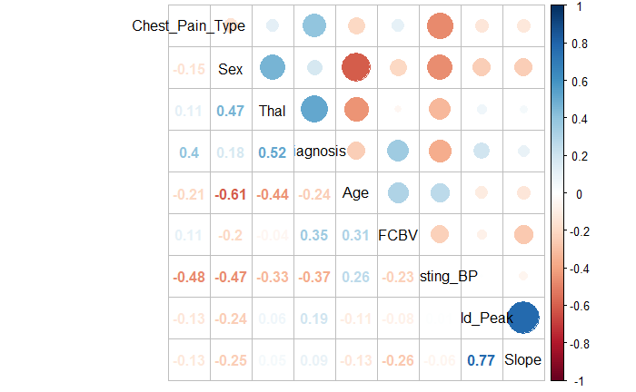

The size and shade of each circle represents the strength of each relationship, while the color represents the direction, either negative or positive. From the plot, there appears to be a strong positive correlation between Old_Peak and Slope. A negative correlation would be Chest_Pain_Type and Resting_BP.

>chart.Correlation(new_data, histogram=T, pch=19)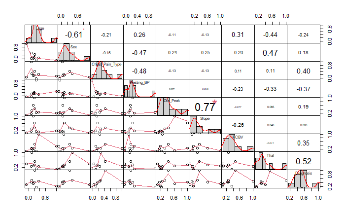

Like the correlation plot, the correlation chart shows the strength of each relationship through charts. The strong positive correlation between Slope and Old_Peak is also high-lighted here and identified to be statistically significant.

#Changing categorical variables to factors

>Heart_data$Sex<-as.factor(Heart_data$Sex)
>Heart_data$Chest_Pain_Type<-as.factor(Heart_data$Chest_Pain_Type)
>Heart_data$High_FBS<-as.factor(Heart_data$High_FBS)
>Heart_data$Resting_ECG<-as.factor(Heart_data$Resting_ECG)
>Heart_data$Ex_Ang<-as.factor(Heart_data$Ex_Ang)
>Heart_data$Slope<-as.factor(Heart_data$Slope)
>Heart_data$FCBV<-as.factor(Heart_data$FCBV)
>Heart_data$Thal<-as.factor(Heart_data$Thal)
>Heart_data$Diagnosis<-as.factor(Heart_data$Diagnosis)

>str(Heart_data)
'data.frame':	270 obs. of  14 variables:
 $ Age            : int  70 67 57 64 74 65 56 59 60 63 ...
 $ Sex            : Factor w/ 2 levels "0","1": 2 1 2 2 1 2 2 2 2 1 ...
 $ Chest_Pain_Type: Factor w/ 4 levels "1","2","3","4": 4 3 2 4 2 4 3 4 4 4 ...
 $ Resting_BP     : int  130 115 124 128 120 120 130 110 140 150 ...
 $ Serum_Cho      : int  322 564 261 263 269 177 256 239 293 407 ...
 $ High_FBS       : Factor w/ 2 levels "0","1": 1 1 1 1 1 1 2 1 1 1 ...
 $ Resting_ECG    : Factor w/ 3 levels "0","1","2": 3 3 1 1 3 1 3 3 3 3 ...
 $ Heart_Rate_Max : int  109 160 141 105 121 140 142 142 170 154 ...
 $ Ex_Ang         : Factor w/ 2 levels "0","1": 1 1 1 2 2 1 2 2 1 1 ...
 $ Old_Peak       : num  2.4 1.6 0.3 0.2 0.2 0.4 0.6 1.2 1.2 4 ...
 $ Slope          : Factor w/ 3 levels "1","2","3": 2 2 1 2 1 1 2 2 2 2 ...
 $ FCBV           : Factor w/ 4 levels "0","1","2","3": 4 1 1 2 2 1 2 2 3 4 ...
 $ Thal           : Factor w/ 3 levels "3","6","7": 1 3 3 3 1 3 2 3 3 3 ...
 $ Diagnosis      : Factor w/ 2 levels "1","2": 2 1 2 1 1 1 2 2 2 2 ...

Simple Linear Regression

Null and Alternative Hypothesis

Null Hypothesis

H0:There will be no significant prediction of Serum_Cho by Age.

Alternative Hypothesis

H1: There will be a significant prediction of Serum_Cho by Age.

>plot(Heart_data$Age, Heart_data$Serum_Cho)
>h<-lm(Serum_Cho~Age, data= Heart_data)
>abline(h, col='red')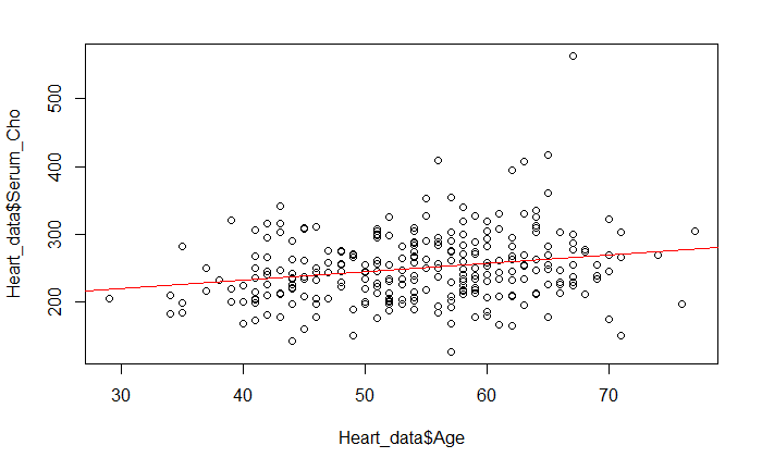

su>summary(h)
##
## Call:
## lm(formula = Serum_Cho ~ Age, data = Heart_data)
##
## Residuals:
## Min 1Q Median 3Q Max
## -126.864 -34.233 -3.756 28.697 298.650
##
## Coefficients:
## Estimate Std. Error t value Pr(>|t|)
## (Intercept) 181.6920 18.6593 9.737 < 2e-16 ***
## Age 1.2486 0.3381 3.693 0.000269 ***
## ---
## Signif. codes: 0 '***' 0.001 '**' 0.01 '*' 0.05 '.' 0.1 ' ' 1
##
8
## Residual standard error: 50.51 on 268 degrees of freedom
## Multiple R-squared: 0.04842, Adjusted R-squared: 0.04487
## F-statistic: 13.64 on 1 and 268 DF, p-value: 0.0002686

There appears to be a positive correlation between Age and Serum_Cho as shown by the statistically significant p-value(0.00026). The estimated mean y value when all x are 0 (Intercept) is also statistically significant.

>par(mfrow=c(2,2))
>plot(h) #Diagnostic Plots

The residuals vs fitted as well as the normal Q_Q plots seem to conform to normality. The Scale_Location does not show homoscedasticity which may need to be investigated further.
Residuals vs Leverage show a few outliers requiring further investigation.

Conclusion

There seems to be a positive linear relationship between Age and Serum_Cho. Higher Serum_Cho levels seem to be associated with older people. I reject the NULL in favor of the alternative hypothesis.